Monte Carlo Simulation
Estimating Pi with Monte Carlo Simulation
import numpy as np
import matplotlib.pyplot as plt
from scipy.stats import norm
circle = plt.Circle((0,0), 1, fill=False)
fig, ax1 = plt.subplots(figsize=(5,5))
ax1.add_artist(circle)
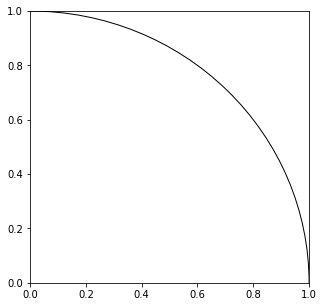
The proportion of the area enclosed by the quadrant to the area enclosed by the square is calculated as,
\[\pi/4 : 1 = \frac{\pi}{4}\]Uniformly scatter a given number of points over the square and count the number of points inside the quadrant. Then, the ratio of the counted number to the number of trials should approximate \(\frac{\pi}{4}\), if the number of trials is large enough. Multiplying this by 4 will give the estimate of \(\pi\).
#np.random.seed(2016033582)
N = 100000 #number of points
x = np.random.uniform(low=0, high=1, size=N) #uniformly distributed x from 0 to 1
y = np.random.uniform(low=0, high=1, size=N) #uniformly distributed y from 0 to 1
x_in = np.array([])
y_in = np.array([])
count = 0
for i in range(N):
if x[i]**2 + y[i]**2 < 1:
x_in = np.append(x_in, x[i])
y_in = np.append(y_in, y[i])
count += 1
pi_estimate = 4 * count / N
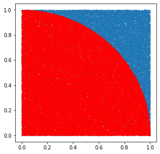
fig, ax2 = plt.subplots(figsize=(5,5))
ax2.scatter(x,y,s=0.5)
ax2.scatter(x_in,y_in,s=0.5,color='r')
print("The estimate of pi for %d trials is %f."%(N,pi_estimate))
The estimate of pi for 100000 trials is 3.139680.
Estimating Call Option Premium with Monte Carlo Simulation
Option Pricing with Monte Carlo Simulation
Simulated stock price, \(S_T\)
\(\tilde{S}_T = S_0e^{(r-\frac{1}{2}\sigma^2)T+\sigma\sqrt{T}\tilde{Z}}\) , where \(\tilde{Z} \sim N(0,1)\)
np.random.seed(2016033582)
N = 100000 #number of runs
Z = np.random.normal(0,1,N) #random number from the standard normal distribution

def stockprice(S0, r, sigma, T, Z):
  """
  S0 : initial stock price
  r : risk-free rate
  sigma : volatility
  T : expiration time
  Z : random number
  """
  S = S0 * np.exp((r - 1/2 * sigma**2) * T + sigma * np.sqrt(T) * Z)
  return S
Call option payoff at expiration, \(\tilde{C}_T\)
\[\tilde{C}_T = \max(S_T - K, 0)\]def calloptionpayoff(S, K):
"""
S : simulated stock price
K : strike price
"""
C = max(S - K, 0)
return C
Given that the current stock price is \(\$50\) with the stock volatility rate of \(20\%\) and the risk free rate of \(2\%\), the call option payoff for the 6-month call with the exercise of \(\$55\), \(\tilde{C}_T\), for each random variable is computed as,
S0 = 50
r = 0.02
sigma = 0.2
T = 0.5

simulated_prices = stockprice(S0, r, sigma, T, Z)
simulated_payoffs = np.array([])

for S in simulated_prices:
  payoff = calloptionpayoff(S, K=55)
  simulated_payoffs = np.append(simulated_payoffs, payoff)

simulated_payoffs
array([0., 0., 0., ..., 6.6015229, 0., 0.])
The expected payoff of the call option, \(E[\tilde{C}_t]\), is,
E = np.mean(simulated_payoffs)
E
1.244666369330442
By discounting the expected payoff of the call option at risk-free rate, the call option value is finally computed as,
\[c = e^{-rT}E[\tilde{C}_T]\]c_estimate = np.exp(-0.02 * 0.5) * E
c_estimate
1.2322817320287849
Comparing with the result from Black Scholes Option Pricing Model
The formula for a call :
\[c = SN(d_1) - Xe^{-rT}N(d_2)\]with
\[d_1 = \frac{\ln(S/K) + (r + 0.5\sigma^2)T}{\sigma\sqrt{T}}, d_2 = d_1 - \sigma\sqrt{T}\]def d1(S0, K, r, sigma, T):
d1 = (np.log(S0/K) + (r + sigma**2 / 2) * T) / (sigma * np.sqrt(T))
return d1
def d2(d1, sigma, T):
d2 = d1 - sigma * np.sqrt(T)
return d2
def BlackScholes(d1, d2, S0, K, r, T):
c = S0 * norm.cdf(d1) - K * np.exp(-r*T) * norm.cdf(d2)
return c
S0 = 50
K = 55
r = 0.02
sigma = 0.2
T = 0.5
d1 = d1(S0, K, r, sigma, T)
d2 = d2(d1, sigma, T)
c = BlackScholes(d1, d2, S0, K, r, T)
c
1.2364710685682443
percent_error = abs(c - c_estimate) / c * 100
print("percent_error : {}%".format(percent_error))
percent_error : 0.33881395577742046%